• sparselizard

    HIGH-PERF C++ FEM LIBRARY

  • sparselizard

    GENERAL NONLINEAR MULTI-PHYSICS

  • sparselizard

    HP-ADAPTIVE (HPFEM)

  • sparselizard

    TRANSIENT EIGENMODE MULTI-HARMONIC

  • sparselizard

    3D 2D 1D + AXISYM

  • sparselizard

    GENERAL MORTAR FEM

  • sparselizard

    GENERAL PERIODIC CONDITIONS

  • sparselizard

    ELECTRIC CIRCUIT COUPLING

  • sparselizard

    INPUT MEASURED PROPERTIES

  • sparselizard

    USER FRIENDLY

  • sparselizard

    OPEN SOURCE

  • sparselizard

    DIRECT LINK TO GMSH API

  • sparselizard

    PYTHON BINDINGS

OVERVIEW

Sparselizard (GNU GPLv2+, Copyright (C) 2020-2021 A. Halbach, Copyright (C) 2018-2019 A. Halbach, IMEC, Copyright (C) 2017 A. Halbach and C. Geuzaine, University of Liege) is a high-performance, multiphysics, hp-adaptive, open source C++ finite element library running on Linux, Mac and Windows. It is carefully validated against analytical solutions, third party software and lab measurements. General high-performance domain decomposition methods are available for large-scale simulations on computing clusters

DDM FOR LARGE SCALE COMMERCIAL SIMULATIONS WITH .ALLSOLVE

For a commercial solution for large-scale multiphysics simulations, check out .allsolve from Quanscient. Built on top of Sparselizard developed by the company CTO Dr. Alexandre Halbach, .allsolve has been enhanced to become the fastest multiphysics solver on the market.

LEARN MORE ABOUT .ALLSOLVE
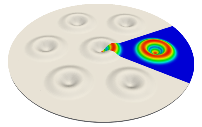
Efficient conformal adaptive mesh refinement (AMR) is provided for 3D, 2D and 1D problems. A fast algorithm for mesh-to-mesh interpolation and a general implementation of the mortar finite element method allow to easily work with non-matching meshes and provide general 
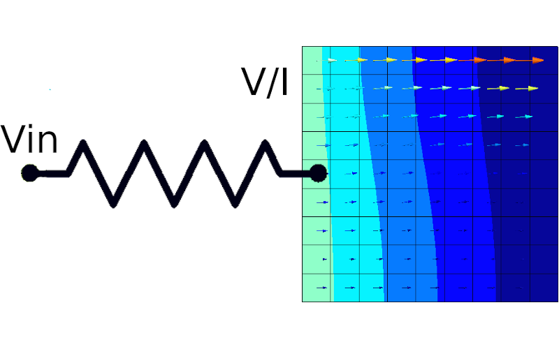
periodic conditions. FEM simulations can be weakly or strongly coupled to lumped electric circuits. Sparselizard can handle a general set of problems in 3D, 2D axisymmetric, 2D and 1D such as 
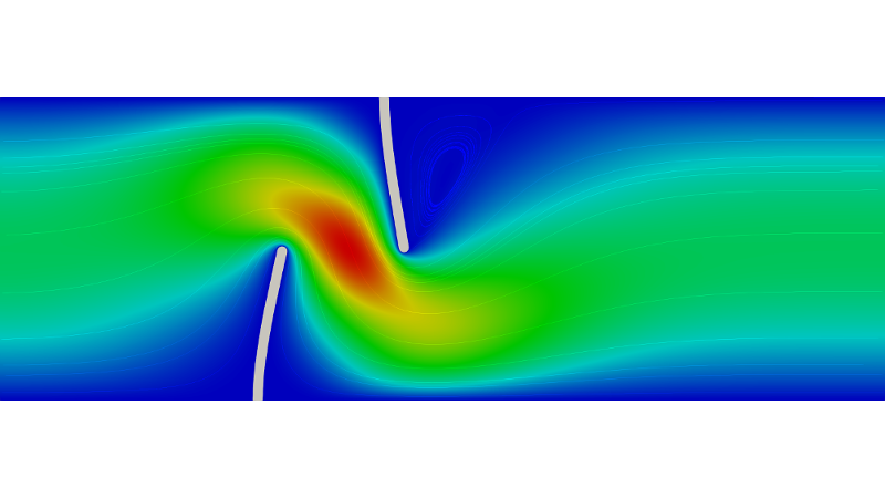
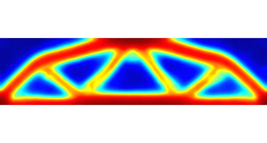
mechanical (anisotropic elasticity, geometric nonlinearity, buckling, contact, crystal orientation), fluid flow (laminar, creeping, incompressible, compressible), stabilized advection-diffusion, nonlinear acoustic, thermal, thermoacoustic, fluid-structure interaction, electric, magnetic, electromagnetic, piezoelectric, superconductor,... problems with a transient, (multi)harmonic or damped/undamped eigenmode analysis. A massive amount of data can be stored for delayed, remote post-processing thanks to the ultra compact .slz data format. Problems with several millions of unknowns in 3D and several tens of millions of unknowns in 2D have been solved within minutes on up to 32 cores/64 threads (see report). Some 
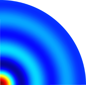
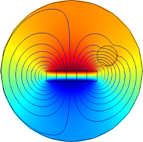
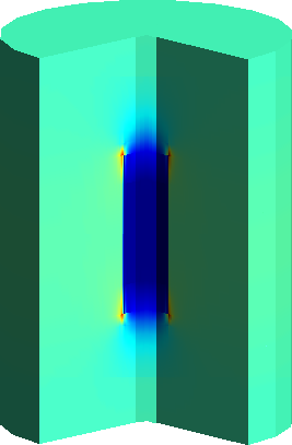
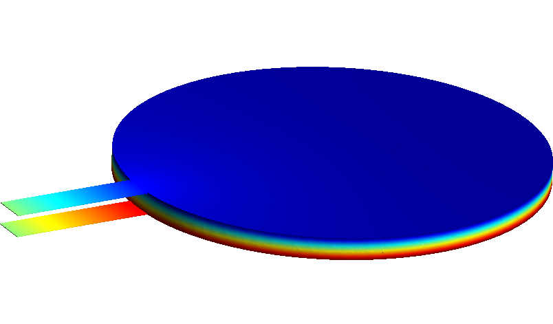
built-in geometry definition and meshing tools are also provided. A working example that solves an electrostatic problem on a grounded 3D disk with electric volume charges can be found below:

int vol = 1, sur = 2;              // Disk volume and boundary as set in ’disk.geo’
mesh mymesh("disk.msh");

field v("h1");                     // Nodal shape functions for the electric potential
v.setorder(vol, 2);                // Interpolation order 2 on the whole domain
v.setconstraint(sur, 0);           // Force 0 V on the disk boundary

formulation elec;                  // Electrostatics with 1 nC/m^3 charge density
elec += integral(vol, -8.854e-12 * grad(dof(v)) * grad(tf(v)) + 1e-9 * tf(v));

elec.solve();                      // Generate, solve and save solution to field v

(-grad(v)).write(vol, "E.vtk", 2); // Write the electric field to ParaView format

The built-in geometry definition and mesher can be used for now for rather simple 2D or extruded 3D geometries. Meshes of complex geometries can be imported from the widely-used open-source GMSH meshing software (.msh format), from Nastran (.nas format) or from various other supported mesh formats (see the mesh object in the documentation). Points, lines, triangles, quadrangles, tetrahedra, hexahedra, prisms or any combination thereof are accepted in the mesh. Element curvature for an accurate representation of the geometry is supported. The result files output by sparselizard are in .vtk / .vtu / .pvd (ParaView) or .pos (GMSH) format. The library comes with hierarchical high order shape functions so that high order interpolations can be used with an interpolation order adapted to every unknown field and mesh element/geometrical region (p-adaptivity).

EXAMPLES

UNSTEADY FLUID FLOW PAST AN OBSTACLE


Von Karman vortex street

The fluid flow past an obstacle is simulated in time with DNS for an increasing inlet velocity. A von Karman vortex street appears at a high enough inlet velocity. The flow can be visualized in time here in 3D and here in 2D.

SEE EXAMPLE

MAGNETIC INDUCTION, SKIN EFFECT


Magnetic induction

An AC voltage is applied to a coil surrounding an aluminium tube in which currents are induced. In the current density cut displayed on the right, the skin effect in the thick copper wire of the coil is clearly visible.

SEE EXAMPLE

SYNCHRONOUS ELECTRIC MOTOR


Piezoresistor - non matching mesh

The induction field and the motor torque of a permanent magnet synchronous electric motor are calculated for an increasing mechanical angle. Only 1/8 of the geometry has to be simulated (anti-periodicity). Follow this link and this link for a visualization video.

SEE EXAMPLE

PIEZORESISTOR, NON MATCHING MESHES


Piezoresistor - non matching mesh

The deflection of a monocrystalline silicon cantilever causes a change in the resistance of the doped (piezoresistive) conducting track in it. The cantilever and track meshes do not match, field interpolation has to be used.

SEE EXAMPLE

FLUID-STRUCTURE INTERACTION


FSI

A pair of micropillars placed in a microchannel bend due to a forced inlet water velocity. Geometric nonlinearity is taken into account in the mechanical model. A Laplace formulation is used to smooth the deformed fluid mesh.

SEE EXAMPLE

OPTICAL WAVEGUIDE COUPLING MODES


Electromagnetic waveguide

The coupling (eigen)modes between two photonic SiN waveguides in a SiO2 cladding are calculated. The waveguide is designed for optical frequencies.

SEE EXAMPLE

FLUID COUPLED PIEZO ACTUATED MEMS


MEMS with fluid coupling

A piezoelectric actuated micromembrane (PMUT) outputs ultrasound pressure waves in air. The simulation is performed in 2D using axisymmetry. Follow this link for a time visualization video of a smilar device (CMUT).

SEE EXAMPLE

TOPOLOGY OPTIMIZATION


Topology optimisation

This mechanical steel structure is automatically optimized to withstand a given force with the minimum possible steel volume. This was obtained with a third-party C++ topology optimization code developed using the sparselizard library for all finite element calculations.

PORTS, ELECTRIC CIRCUIT COUPLING


Electric circuit coupling

Lumped electric circuit elements can be accurately calculated from a FEM simulation or coupled to it in a strong or weak way. Additional lumped operations like computing mechanical reaction forces can be treated with the same tools.

R CALCULATION RLC TRANSIENT C CALCULATION RLC HARMONIC

PERMANENT MAGNETS, MAGNETIC FORCE


Permanent magnets

The static magnetic field created by an array of permanent magnets is simulated using the scalar magnetic potential formulation. The Halbach configuration shows as expected a magnetic field strength increase. The potential and the magnetic field lines are illustrated.

SEE EXAMPLE

HALF-WAVE DIPOLE ANTENNA


Half-wave dipole antenna

The 1 GHz electromagnetic wave radiation of a half-wave dipole antenna is simulated. The electric field, magnetic field and Poynting vector are computed and can be visualized in time. The electric field can be visualized here.

SEE EXAMPLE

GENERAL PERIODIC CONDITIONS


Periodic condition

The crosstalk between a central micromembrane and 6 neighbours is analyzed on only 1/6 of the geometry using a periodic condition between two faces with non-matching meshes. The available mortar finite element method allows to implement general periodic conditions.

SEE EXAMPLE

HIGH TEMPERATURE SUPERCONDUCTOR


High temperature superconductor

A thin superconducting tube is subject to an applied magnetic field that increases over time. As the magnetic field is increased it progressively penetrates in the tube until the tube is not able to perfectly shield its interior volume anymore. The time-solution can be visualized here.

SEE 2D EXAMPLE SEE 3D EXAMPLE

INFLUENCE OF SI/PZT CRYSTAL ORIENTATION


Piezoelectric micro-bilayer

A piezoelectric PZT layer grown on a monocrystalline silicon wafer is sandwiched between two electrically actuated electrodes, creating a harmonic deflection of the bilayer. The crystal orientation of both the PZT and the silicon can be changed to any direction. Follow this link for a time visualization video.

SEE EXAMPLE

DAMPED MECHANICAL RESONANCE MODES


Mechanical disk eigenmodes

The damped eigenmodes and eigenfrequencies are obtained for a 3D disk clamped at its side. A proportional damping is used to model losses.

SEE EXAMPLE

CONDUCTOR HEATING DUE TO DC CURRENT


Conductor heating due to DC current

A voltage is applied across a 3D tungsten conductor in vacuum. The (strong) DC current flow as well as the induced thermal heating (displayed) is simulated. The influence of the temperature on the material properties is taken into account with a nonlinear loop.

SEE EXAMPLE

ELECTROMAGNETIC WAVEGUIDE


Electromagnetic waveguide

A cross shaped perfectly conducting 3D waveguide is excited with an imposed electric field at one end. Follow this link for a transient time resolution video.

SEE EXAMPLE

MAGNETIC STRESSES, MAGNETOSTRICTION


Magnetostriction

The magnetic stress state created by a DC current flow in a choke (inductor) is computed. The corresponding mechanical deformation is deduced. Magnetostrictive stresses are taken into account.

SEE EXAMPLE

STATIC MAGNETIC SATURATION


Magnetic saturation

A magnetic steel shell surrounds two insulated copper conductors with DC currents flowing in opposite directions. For large currents the shell is saturated. An iterative resolution of the A-v formulation is used to solve this nonlinear problem.

SEE EXAMPLE

A-V AND H-PHI FORMULATION


H-phi formulation

The magnetic field and induction created by AC currents in three wires is simulated using an A-v and a H-phi formulation. Cohomology cuts are required in the H-phi case. The picture shows the magnetic induction field, the current density in each wire and the cuts.

SEE AV EXAMPLE SEE HPHI EXAMPLE

WORKING WITH EXPERIMENTAL DATA


Experimental data

The deflection of a steel disk with a non-uniform temperature profile is calculated: the stiffness versus temperature dependence is obtained by interpolating between experimental data samples using natural cubic splines.

SEE EXAMPLE

THERMOACOUSTICS IN A DEFORMABLE CAVITY


Transient thermoacoustic

The transient thermoacoustic response to a 0.1 us laser pulse in a 500 um deformable cavity with ambient air on top is simulated. The fields displayed are the fluid pressure, velocity, temperature and membrane deformation. Follow this link for a time visualization video.

SEE EXAMPLE

BUCKLING, GEOMETRIC NONLINEARITY


MEMS with fluid coupling

A prestressed 3D bilayer micromembrane is pushed downwards by the atmospheric pressure. The static deflection and resonance frequency shift is simulated thanks to a small-strain geometric nonlinearity formulation. This example can be adapted to simulate buckling in time, as shown in this video.

SEE EXAMPLE

POTENTIAL AIR FLOW AROUND AN AIRFOIL


Potential air flow around an airfoil

A NACA0012 airfoil is put in a subsonic air flow. The problem is nonlinear because the air density is a function of the air speed. The picture shows the Mach number everywhere around the airfoil.

SEE EXAMPLE

NATURAL CONVECTION,
HP-ADAPTIVITY


Natural convection in air

The natural convection created by a hot disk in a colder air environment is simulated using hp-adaptivity. The fully compressible flow is considered and solved in time. Follow this link, this link and this link for a time visualization video.

SEE EXAMPLE

CONTACT MECHANICS, COLLAPSED CMUT


Collapsed CMUT

The collapse mode of a CMUT ultrasonic transducer is simulated (in collapse mode the membrane touches the bottom of the cavity). The static deflection as well as the small signal vibration are simulated and illustrated on the image. The collapse mode of a CMUT can be visualized here (vibration in a fluid) and here (static collapse).

SEE EXAMPLE

RESISTANCE AND CAPACITANCE


RC simulation

The resistance and capacitance is computed for a 3D geometry made of a conducting trace connected to a circular-shaped, parallel-plate air capacitor. The simulated capacitance matches the parallel plate formula. The quadrature electric potential field is displayed on the picture above.

SEE EXAMPLE

STABILIZED ADVECTION DIFFUSION


Stabilized advection-diffusion

This is a sandbox example for stabilized (advection dominated) advection-diffusion problems. The isotropic, streamline anisotropic, SPG, SUPG, crosswind and crosswind-shockwave stabilization methods are predefined.

SEE EXAMPLE

MAGNETIC SHIELDING OF A DC CURRENT


Magnetic shielding of a DC current

A 3D steel cylinder is placed nearby a wire with a given static current density. The magnetic vector potential formulation is used. A gauge condition is added in combination with a spanning tree to remove the singular matrix problem associated with the formulation.

SEE EXAMPLE

DOUBLE DIFFUSION OF SALT FINGERS


Double diffusion

A coupled thermal-salt concentration advection-diffusion problem is simulated in time in presence of a gravity force. The picture shows the appearing salt fingers as well as the density inversion phenomenon.

DIRECT LINK
TO GMSH API


Stabilized advection-diffusion

This example shows how to load to sparselizard a mesh created with the GMSH API. Linking to this API is optional but provides powerful CAD and meshing support.

SEE EXAMPLE

LAMINAR FLOW,
HP-ADAPTIVITY


Laminar flow

The nonlinear Navier-Stokes equations for incompressible laminar flow are solved with a Newton iteration to simulate the water flow past a step in a 1 mm pipe. HP-adaptivity is used. The top image is the flow velocity, the bottom image is the adapted mesh.

SEE EXAMPLE

FLUID FLOW IN A MICROVALVE


Fluid flow in a microvalve

The flow speed magnitude (top) and the pressure field (bottom, 100 Pa at left inlet and 0 Pa at right outlet) are computed for a low Reynolds (Stokes) flow in a microvalve.

SEE EXAMPLE

ELECTRIC MOTOR,
P-ADAPTIVITY


Double diffusion

The interpolation order (right) in this PMSM magnetic field simulation is adapted to every mesh element based on an input criterion (e.g. field gradient). For a given accuracy this speeds up the simulation since the computational effort is added only where needed. Visualization here.

SEE EXAMPLE

DOWNLOAD

The easiest way to get the sparselizard finite element library running on Linux and Windows 10 is to use its C++ static library (recommended). Alternatively you can manually compile it on your computer.
Get sparselizard running with one of the following options:

Windows 10, Mac, Linux - Python bindings
  • Compile spylizard, the sparselizard python bindings
Windows 10, Mac, Linux - Compiling the C++ source code
  • Download the source code here
  • Follow the instructions in the documentation
  • For Visual Studio on Windows 10 follow this link
  • For Visual Studio on Windows 10 Linux subsystem a step-by-step procedure is available upon request
  • More info about Windows Linux subsystem can be found here
  • (more info on how to access files from each side here)
Linux - C++ static library (TUTORIAL VIDEO)
  • Watch the tutorial video
  • Download the static library here and open the folder in a terminal.
  • Run 'g++ -O3 -fopenmp -std=c++11 -Wno-return-type -fPIC -no-pie main.cpp -L ./ -l sparselizard -pthread -l dl -I headers -o slexe;'
  • Run './slexe'
  • Visualise the output .vtk file with ParaView
Windows, Mac, Linux - Docker (in progress) Windows 10 - C++ static library with Linux subsystem
  • Watch the tutorial video for Linux
  • Install an Ubuntu subsystem on Windows 10 as detailed here
  • (more info on how to access files from each side here)
  • Download the static library here using 'wget' to the Ubuntu subsystem
  • Run 'sudo apt-get install unzip' then unzip the file
  • Run 'sudo apt-get install g++' to install the C++ compiler
  • In the unzipped file run 'g++ -O3 -fopenmp -std=c++11 -Wno-return-type -fPIC -no-pie main.cpp -L ./ -l sparselizard -pthread -l dl -I headers -o slexe;'
  • Run './slexe'
  • Visualise the output .vtk file with ParaView. This has to be done on Windows unless graphics are supported in your subsystem
Windows (others), Mac - Virtual Linux machine
  • A virtual Ubuntu Linux can be easily installed using VirtualBox.

Follow the applied FEM lectures, take a look at the examples in the 'examples' folder and at the documentation for a smooth introduction.

CITE US / DONATE

Because sparselizard is free and open source does not mean lines of code appear magically without effort. This library was partly developed unpaid, after work. Even more to that, the web hosting costs and domain name costs are fully supported by myself. When using sparselizard cite reference:
HALBACH, Alexandre. Sparselizard-the user friendly finite element c++ library. 2017.


CONTACT

It would be a pleasure to answer any of your questions or to get your bug reports.
In the latter case please provide a minimal code including the bug.

Alexandre Halbach

ALEXANDRE HALBACH


PhD - Electrical Engineering

alexandre.halbach at gmail.com